
Market equilibrium is a situation in which the quantity buyers plan to purchase equals the quantity sellers plan to offer at a particular price. In the basic competitive model, that price is the equilibrium or market-clearing price, and the corresponding amount traded is the equilibrium quantity.
The condition concerns a defined product, market and period. It does not mean that everyone can afford the product, every seller earns a profit or every available physical item must be sold.
Price and quantity work together
Demand describes how planned purchases vary across prices, other things equal. Quantity demanded is the amount wanted and affordable at one price. Supply likewise describes planned sales across prices; quantity supplied refers to one price.
The OpenStax explanation introduces the competitive equilibrium model. On the usual diagram, price is vertical and quantity per period is horizontal. The intersection identifies both values.
A market’s equilibrium is therefore not merely another name for its price. It is the combination of compatible buying and selling plans under the model’s conditions.
A worked market example
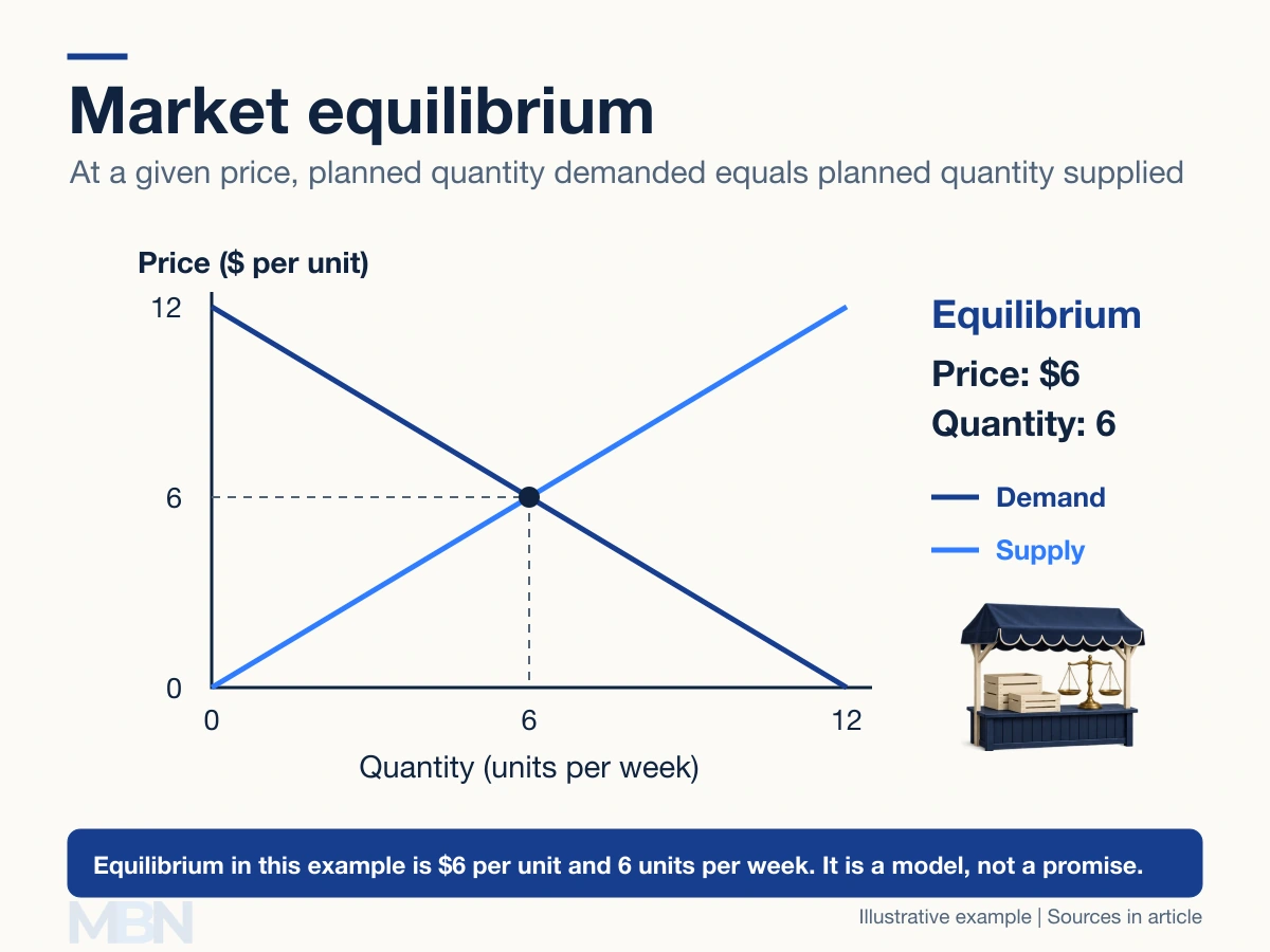
Imagine a weekly market with these illustrative schedules: quantity demanded = 12 − price, and quantity supplied = price. Price is measured in dollars per unit and quantity in units per week.
Equating them gives 12 − price = price, so price = $6. At that price, buyers want six units and sellers offer six units. Their plans match.

At $4, buyers want eight units while sellers offer four, leaving excess demand of four units. At $8, buyers want four units while sellers offer eight, leaving excess supply of four units.
These gaps compare plans at the specified price. They are not necessarily actual completed trades or a count of inventory already manufactured.
Why prices may adjust
In the flexible-price model, a shortage gives sellers scope to raise prices, while unsold offers can create pressure to lower them. Price changes alter quantities along the existing schedules.
Adjustment need not be immediate or smooth. Contracts, delivery times, search costs, inventories, bargaining and regulations can slow it. A single-crossing diagram does not establish that every real market has one unique, stable equilibrium.
The textbook discussion of price ceilings and floors shows how binding controls can prevent clearing in this model. A ceiling below $6 would create a shortage in the example; a ceiling above $6 would not constrain the original equilibrium price.
Movement versus a new equilibrium
A change in the product’s own price causes movement along a given demand or supply curve. A change in another influence can shift a curve, producing a different equilibrium.
For example, lower production costs can increase the quantity sellers offer at each price. With demand unchanged, the basic model predicts a lower equilibrium price and a larger quantity. Stronger demand, with supply unchanged, raises both. The textbook explanation of shifts describes these conditions.
If both curves move, their relative movements matter. The result cannot always be determined from the direction of one shift alone.
Equilibrium does not mean an ideal outcome
Under specific competitive assumptions, equilibrium can exhaust mutually beneficial trades. The discussion of efficiency explains this benchmark. It does not establish that the resulting distribution is fair or that everyone’s needs are met.
Market prices may also omit costs imposed on others, such as pollution. These externalities can make a private market’s equilibrium differ from the socially efficient outcome, as the pollution example explains.
Equilibrium is useful for organizing a question about prices, quantities and changes in conditions. Its conclusions remain tied to the assumptions and evidence used for the particular market.
Last checked and updated on November 11, 2026 by the MBN editorial team.